All Resources
R-45
Technology
How Graph Databases Actually Walk Your Data
Adjacency lists, CSR matrices and hash-indexed traversal — the three ways engines store relationships and follow them, with one small graph traced through each.
PAR2 Labs
September 16, 2026
12 min
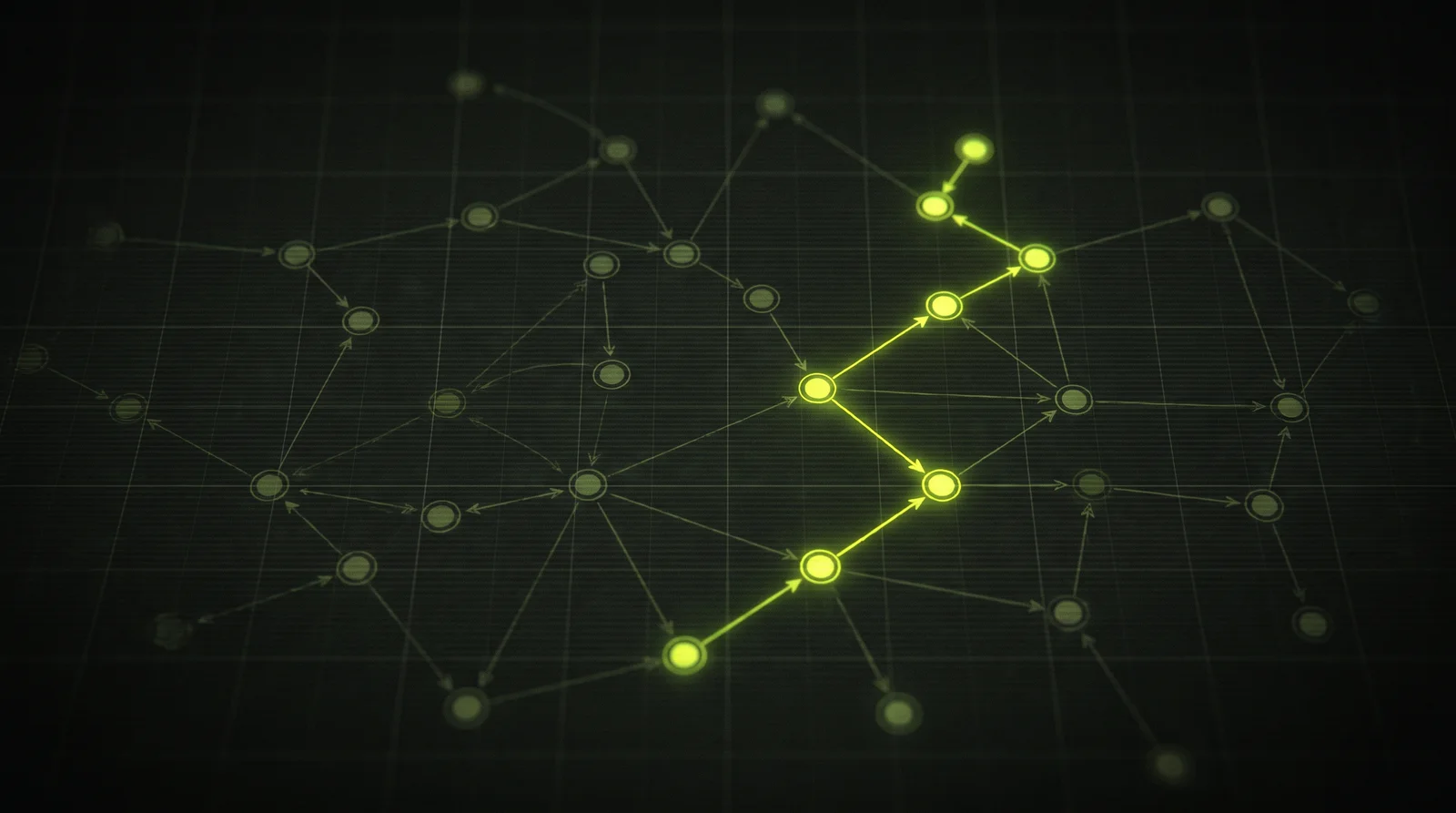
Every graph database sells the same promise: it can answer “how are these things connected?” far faster than a relational database, and it stays fast as the data grows. That promise doesn't come from magic — it comes from how the engine physically stores relationships and follows them.
Watch the explainer
4:57
Narrated end to end. The same five-node graph is traced through all three designs, each one drawn as it is explained.
01
First, the vocabulary: V and E
V = vertices (the nodes — accounts, people, devices). E = edges (the relationships — transactions, shared attributes). Two cost expressions decide everything.
O(V + E) is work proportional to nodes plus edges. You add them because a full traversal touches each node once and each edge once. Sparse storage designs live here. O(V²) is work proportional to nodes times nodes: one slot for every possible pair, whether an edge exists or not. Dense-matrix storage lives here.
Why the gap matters
01
For a graph of 1,000,000 nodes averaging 100 links each, V + E ≈ 101 million (~10⁸), while V² = 10¹² — roughly 10,000× larger.
02
99.99% of those cells would be empty. Real graphs are sparse, which is exactly why no serious engine stores one as a dense grid.
02
The example graph
Five accounts (IDs 0–4), directed “PAID” edges. Our test hop everywhere: give me the direct neighbours of node 0 — the answer must be 1 and 2.
There is a cycle (0→1→3→0), a second path to the same node (0→2→3), and one account with no edges at all. Node 4 is there on purpose: an isolated vertex is where storage designs differ most visibly.
The same graph is traced through all three storage designs. Node 0's two out-edges are the hop being measured.
03
Method 1 — Adjacency list, the Neo4j school
The idea is the one you would reach for first: each node keeps a list of its own neighbours. Storage is an array of V slots plus E total entries, so O(V + E).
The hop has three steps. Jump to array slot [0] by direct arithmetic — address = base + 0 × slotSize, O(1), no searching. Follow that slot's pointer to its neighbour list. Scan it: 1, 2. That scan is O(degree).
Neo4j does this with fixed-size records in store files, so recordAddress = id × recordSize — which is why dense integer IDs matter. A node record points to its first relationship record, and relationship records form a doubly-linked list. Listing a node's edges means jumping to its record and walking that chain with no index consulted. That is index-free adjacency, and enumeration costs O(degree).
O(V + E) storage. The array gives O(1) access to the node; the list gives O(degree) enumeration.
04
Method 2 — Adjacency matrix, and why CSR replaces it
A dense adjacency matrix is a V × V grid where cell[from][to] = 1 if that edge exists. For our graph that is 5 × 5 = 25 cells to hold 5 edges — O(V²), with only the diagonal-scattered handful filled. Reading node 0's neighbours means scanning its whole row, all V cells, which is O(V) and worse than an adjacency list for sparse data.
But the dense form has a superpower worth keeping. Multiply the matrix by itself and A × A = A² gives two-hop reachability, where A²[i][j] is the number of length-2 paths from i to j. In our graph A²[0][3] = 2 — exactly the two paths 0→1→3 and 0→2→3. “Expand k hops from every node at once” becomes Aᵏ, which CPUs and GPUs run in massively parallel fashion. This is the engine behind whole-graph algorithms like PageRank.
The dense form: every possible pair gets a slot whether an edge exists or not. The empty cells are the cost.
05
CSR — keep the superpower, drop the O(V²) waste
Compressed Sparse Row stores only the non-zeros in two flat arrays. col_index[] holds every neighbour, row by row, concatenated. row_ptr[] holds where each row starts, and has length V+1 so the last entry closes the final row.
The hop becomes two O(1) reads and a scan: start = row_ptr[0] = 0, end = row_ptr[1] = 2, then read col_index[0..2) = [1, 2]. Node 4 resolves to col_index[5..5), an empty slice, without storing anything for it.
Storage is back to O(V + E) and fully contiguous — the best cache behaviour of any method here — and you can still run the matrix multiply as sparse matrix–vector products. The catch is writes: inserting one edge shifts col_index and bumps every later row_ptr, so CSR is rigid to mutate.
Two flat arrays replace the grid. The slice between consecutive row_ptr entries is the node's neighbour list.
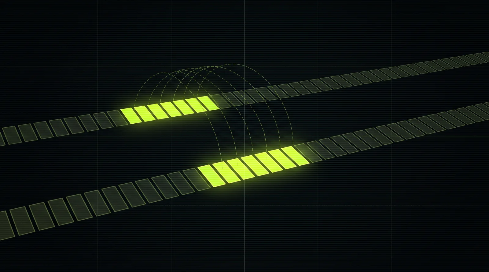
Why CSR reads fast: the neighbours of a node are adjacent in memory, so one cache line often carries the whole list.
06
Method 3 — Hash-indexed adjacency, the Tessera school
Same “node → its neighbours” idea, but the node's identity is a Multihash — a 34-byte, content-addressed hash — not a dense integer. You cannot index an array with a 34-byte hash, so you hash it and look it up in a map. Tessera nests three levels: node → relationship-type → a contiguous list of (neighbour, edge) pairs.
The hop is two lookups and a scan. Hash the node ID to find its bucket in the outer map and get the inner map. Hash the relationship type — “PAID” — to get the Vec. Then scan the Vec of (neighbour, edge) pairs, which is O(degree) over a contiguous leaf.
The trade-off is honest: the scan is the same O(degree) as everyone else, and the difference is in the lookup. Array indexing is O(1) arithmetic with perfect locality, while hashing pays real CPU cost over 34 bytes and lands in scattered buckets. In exchange, content-addressed IDs give global uniqueness without a central allocator, deduplication, integrity and verifiability, coordination-free merging, and — because the edge ID sits in the leaf — edges as first-class addressable entities, which is what a hypergraph or provenance engine needs. The middle relationship-type layer also makes typed traversal free: follow only PAID, and the other types are never touched.
Typed traversal comes free from the middle layer: asking for one relationship type never touches the others.
07
The differences, side by side
All three sparse designs are O(V + E) to store and O(degree) per hop — the same complexity class. They differ only in how a node's neighbour list is found, and in what that choice costs and buys.
| Aspect | Adjacency list (Neo4j) | CSR matrix (FalkorDB) | Hash-indexed (Tessera) |
|---|---|---|---|
| Node identity | Dense integer ID | Dense integer index | Multihash — content-addressed, 34 bytes |
| Find a node's list | ID × record size = direct offset | row_ptr array read | Hash the ID, look it up in a HashMap |
| One hop | Follow pointer, walk relationship chain | Read row slice, scan contiguously | 2 hash lookups, then scan the leaf Vec |
| Storage cost | O(V + E) | O(V + E) | O(V + E) |
| Per-hop cost | O(degree) | O(degree) | O(degree) |
| Cache locality | Medium | Best — fully contiguous | Leaf contiguous; maps scattered |
| Mutation / writes | Moderate, OLTP-friendly | Rigid — rebuild or delta | Cheapest — insert anywhere |
| Superpower | Index-free adjacency | Traversal = matrix multiply (Aᵏ) | Global IDs, edges as first-class entities |
| Best for | General OLTP graph workloads | Whole-graph analytics and sweeps | Write-heavy, hypergraph, verifiable |
Same complexity class throughout. The differences are constant factors and write behaviour — which is where real workloads live.
08
So which is best?
None absolutely — each is a different point on the same trade-off curve, and the honest answer is workload-dependent.
The decisive question is never “which is fastest?” but “fastest at what, under whose write pattern?” For targeted traversal from a known starting node — the common fraud, AML and recommendation workload — all three touch only a bounded neighbourhood, so the gap between them is at its smallest. The differences widen at the extremes: whole-graph sweeps favour CSR, high-churn writes favour the hash map, and everyday mixed workloads favour the adjacency list.
A mature architecture often keeps two representations at once — a mutation-friendly store for live reads and writes, and a CSR projection built on demand for heavy analytics. That is exactly what Neo4j does with its transactional store plus an in-memory GDS projection.
Relationships as first-class, cheap-to-follow structures are the whole point of a graph database. Adjacency lists, CSR matrices and hash-indexed maps are simply three ways to deliver that, tuned for reads, analytics and writes respectively.
PAR2 Labs · Technology
Work With Us